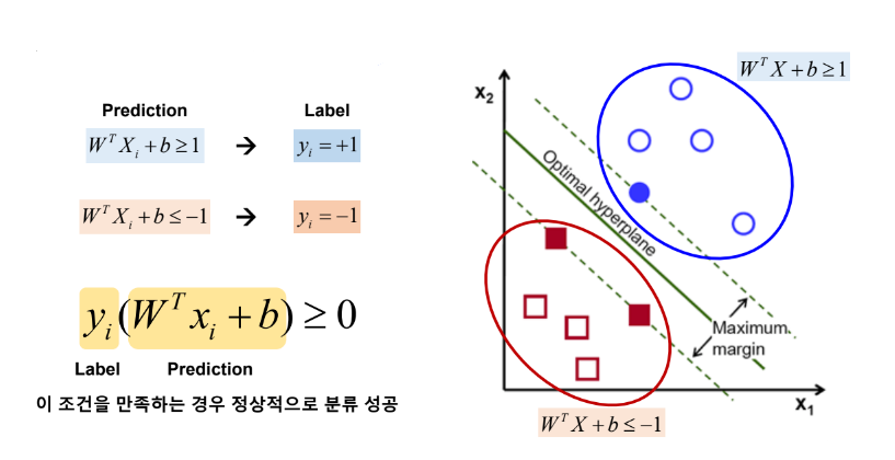
목적 : Margin을 최대화하는 optimal separating hyperplane 구하기
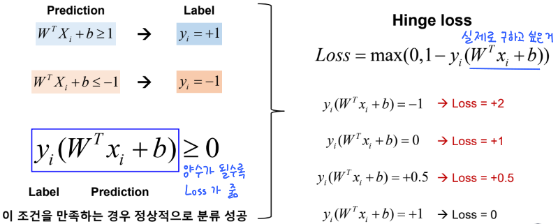
● Loss function 으로 Hinge loss 를 사용
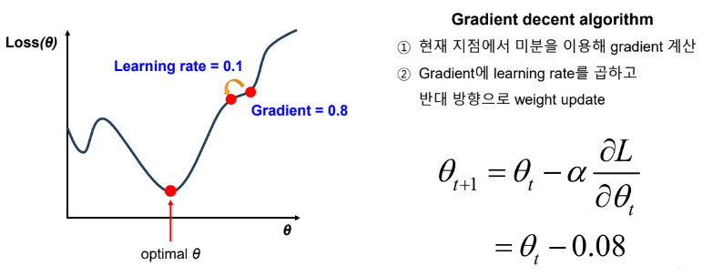
● Hinge loss 으로 Gradient 를 구해야 함

Support Vector Machine (GD Method)
▼ 패키지 선언
import pandas as pd
import numpy as np
import matplotlib.pyplot as plt

from sklearn.datasets import make_blobs
▼ Dataset 생성
X, y = make_blobs(n_samples=50, n_features=2, centers=2, cluster_std=1.05, random_state=40)
plt.scatter(X[:, 0], X[:, 1], marker='o', c=y, s=100, edgecolor="k", linewidth=1)
plt.xlabel("x_1")
plt.ylabel("x_2")
plt.show()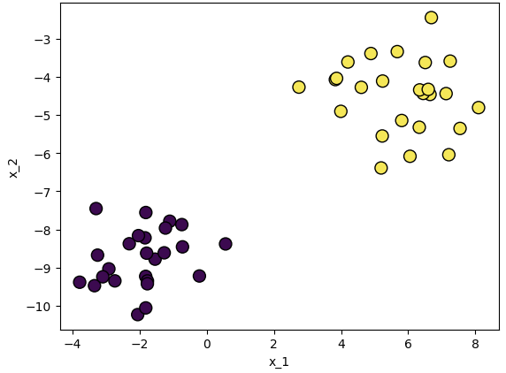
▼ SVM 모델 정의 및 gradient decent 코드 작성
class SVM:
    def __init__(self, learning_rate=0.001, n_iters=1000):
        # initialization
        self.lr = learning_rate
        self.n_iters = n_iters
        self.w = None
        self.b = None


    def fit(self, X, y):
        # Update parameters
        y_ = np.where(y <= 0, -1, +1)
        n_samples, n_features = X.shape
        self.w = np.zeros(n_features)
        self.b = 0

        for i in range(self.n_iters):
          for idx, x_i in enumerate(X):
            condition = y_[idx] * (np.dot(x_i, self.w) + self.b) >= 1

            if not condition:
              self.w -= self.lr * (- np.dot(x_i, y_[idx]))
              self.b -= self.lr * (y_[idx])


    def predict(self, X):
        # Prediction
        prediction = np.dot(X, self.w) + self.b
        prediction = np.sign(perdiction) # 0보다 작으면 -1로 크면 1로 매핑하는 함수이다
        return prediction
▼ SVM 모델 training 및 도출된 W, b 값 확인
model = SVM()
model.fit(X, y)

print(model.w, model.b)
더보기
[0.63613331 0.15767898] -0.06500000000000004
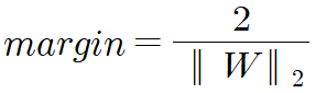
margin = 2 / np.sqrt(np.dot(model.w.T, model.w))
print(margin)
더보기
3.051645856880161
▼ Visualization
def get_hyperplane_value(x, w, b, offset):
    return (-w[0] * x - b + offset) / w[1]

def visualize_svm(w, b):
    fig = plt.figure()
    ax = fig.add_subplot(1, 1, 1)
    plt.scatter(X[:, 0], X[:, 1], marker="o", c=y)

    x0_1 = np.amin(X[:, 0])
    x0_2 = np.amax(X[:, 0])

    x1_1 = get_hyperplane_value(x0_1, w, b, 0)
    x1_2 = get_hyperplane_value(x0_2, w, b, 0)

    x1_1_m = get_hyperplane_value(x0_1, w, b, -1)
    x1_2_m = get_hyperplane_value(x0_2, w, b, -1)

    x1_1_p = get_hyperplane_value(x0_1, w, b, 1)
    x1_2_p = get_hyperplane_value(x0_2, w, b, 1)

    ax.plot([x0_1, x0_2], [x1_1, x1_2], "y--")
    ax.plot([x0_1, x0_2], [x1_1_m, x1_2_m], "k")
    ax.plot([x0_1, x0_2], [x1_1_p, x1_2_p], "k")

    x1_min = np.amin(X[:, 1])
    x1_max = np.amax(X[:, 1])
    ax.set_ylim([x1_min - 3, x1_max + 3])
    plt.xlabel("x_1")
    plt.ylabel("x_2")
    plt.show()
visualize_svm(model.w, model.b)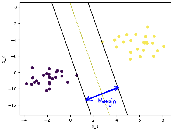
▼ scikit-learn 라이브러리를 이용한 SVM
from sklearn.svm import SVC
model = SVC(kernel='linear')
model.fit(X, y)
visualize_svm(model.coef_[0], model.intercept_)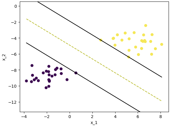
margin = 2 / np.sqrt(np.dot(model.coef_[0].T, model.coef_[0]))
print(margin)
더보기
4.5366449473146595
'머신러닝' 카테고리의 다른 글
| K-Nearest Neighbor (KNN) (0) | 2023.12.18 |
|---|---|
| Entropy (0) | 2023.12.18 |
| Support Vector Machine : Quadratic Programming(2차 계획법) (0) | 2023.12.18 |
| MNIST Classification using SLP, MLP (1) | 2023.12.17 |
| [머신러닝] Loss Function, Optimization, Batch size (2) | 2023.11.24 |


